Next: Building JavaFX applications, Up: Miscellaneous topics [Contents][Index]
Composable pictures
The (kawa pictures) library lets you create geometric shapes
and images, and combine them in interesting ways.
The tutorial gives an introduction.
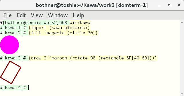
The easiest way to use and learn the pictures library
is with a suitable REPL. You can use the old Swing-based console
or any DomTerm-based terminal emulator.
You can create a suitable window either by starting kawa
with the -w flag, or by running the kawa command
inside an existing DomTerm-based terminal emulator.
The screenshot below is of the latter,
using the qtdomterm terminal emulator.
After (import (kawa swing)) you can use show-picture
to display a picture in a Swing window.
A picture is an object that can be displayed on a screen, web-page, or printed page, and combined with other pictures.
A picture has a method printing itself in a graphical context. It also has various properties.
An important property of a picture is its bounding box. This is a rectangle (with edges parallel to the axes) that surrounds the contents of the picture. Usually the entire visible part of the picture is inside the bounding box, but in some cases part of the picture may stick outside the bounding box. For example when a circle is drawn (stroked) with a “pen”, the bounding box is that of the infinitely-thin mathematical circle, so “ink” from the pen that is outside the circle may be outside the bounding box.
A picture has an origin point corresponding to the (0 0) cordinates.
The origin is commonly but not always inside the bounding box.
Certain operations (for example hbox) combine pictures by putting
them “next to” each other, where “next to” is defined in
terms of the bounding box and origin point.
- Coordinates - points and dimensions
- Shapes
- Colors and paints
- Filling a shape with a color
- Stroking (outlining) a shape
- Affine transforms
- Combining pictures
- Images
- Compositing - Controlling how pictures are combined
- Displaying and exporting pictures
Coordinates - points and dimensions
The library works with a two-dimensional grid, where each position has an x cordinate and y coordinate. Normally, x values increase as you move right on the screen/page, while y values increase as you move down. This convention matches that used by Java 2D, SVG, and many other graphics libraries. However, note that this is different from the traditional mathematical convention of y values increasing as you go up.
By default, one unit is one “pixel”. (More precisely,
it is the px unit in the CSS specification.)
- Type: Point 
A point is a pair consisting of an x and a y coordinate.
- Literal: &P
[x y]¶ Construct a point value with the specified x and y values. Both x and y are expressions that evaluate to real numbers:
&P[(+ old-right 10) baseline]
- Type: Dimension 
A dimension value is a pair of a width and a height. It is used for the size of pictures in the two dimensions.
In a context that expects a point, a dimension is treated as an offset relative to some other point.
- Literal: &D
[width height]¶ Construct a dimension value with the specified width and height values, which are both expressions that evaluate to real numbers.
Shapes
A shape is a collection of lines and curves. Examples include lines, circles, and polygons. A shape can be stroked, which you can think of as being drawn by a very fancy calligraphic pen that follows the lines and curves of the shape.
A closed shape is a shape that is continuous and ends up where it started. This includes circles and polygons. A closed shape can be filled, which means the entire “interior” is painted with some color or texture.
A shape is represented by the Java java.awt.Shape interface.
The picture library only provides relatively simple shapes,
but you can use any methods that create a java.awt.Shape object.
Shape is effectively a sub-type of picture,
though they’re represented using using disjoint classes:
If you use a shape where a picture is required,
the shape is automatically converted to a picture,
as if using the draw procedure.
- Procedure: line p1 [p2 ...] 
In the simple case two points are specified, and the result is a line that goes from point p1 to p2. If n points are specied, the result is a polyline: a path consisting of n-1 line segments, connecting adjacent arguments. (If only a single point is specified, the result is degenerate single-point shape.)
All of the points except the first can optionally be specified using a dimension, which is treated an an offset from the previous point:
(line &P[30 40] &D[10 5] &D[10 -10])
is the same as:
(line &P[30 40] &P[40 45] &P[50 35])
- Procedure: polygon p1 [p2 ...] 
Constructs a closed shape from line segments. This is the same as calling
linewith the same arguments, with the addition of a final line segment from the last point back to the first point.
- Procedure: rectangle p1 [p2] 
A rectangle is closed polygon of 4 line segments that are alternatively parallel to the x-axis and the y-axis. I.e. if you rotate a rectangle it is no longer a rectangle by this definition, though of course it still has a rectangular shape. If p2 is not specified, constructs a rectangle whose upper-left corner is
&P[0 0]and whose lower-right corner is p1. If p2 is specified, constructs a rectangle whose upper-left corner is p1 and whose lower-right corner is p2. If p2 is a dimension it is considered a relative offset from p1, just like forpolygon.
- Procedure: circle radius [center] 
Creates a circle with the specified radius. If the center is not specified, it defaults to
&P[0 0].
Colors and paints
A paint is a color pattern used to fill part of the canvas. A paint can be a color, a texture (a replicated pattern), or a gradient (a color that gradually fades to some other color).
A color is defined by red, green, and blue values. It may also have an alpha component, which specifies transparency.
- Procedure: ->paint value 
Converts value to a color - or more general a paint. Specificlly, the return type is
java.awt.Paint. The value can be any one of:- A
java.awt.Paint, commonly ajava.awt.Color. - A 24-bit integer value is converted to a color.
Assume the integer is equal
to a hexadecimal literal of the form
#xRRGGBB. ThenRR(bits 16-23) is the intensity of the red component;GG(bits 8-15) is the intensity of the green component; andRR(bits 0-7) is the intensity of the red component. - One of the standard HTML/CSS/SVG color names, as a string or symbol.
See the table in
gnu/kawa/models/StandardColor.javasource file. Case is ignored, and you can optionally use hyphens to separate words. For example'hot-pink,'hotpink, and'hotPinkare all the same sRGB color#xFF69B4.
- A
- Procedure: with-paint paint picture 
Create a new picture that is the “same” as picture but use paint as the default paint. For paint you can use any valid argument to
->paint. The default paint (which is the color black if none is specified) is used for bothfill(paint interior) anddraw(stroke outline).#|kawa:1|# (! circ1 (circle 20 &P[20 20])) #|kawa:2|# (hbox (fill circ1) (draw circ1)) [ images/paint-circ-1 ] #|kawa:3|# (with-paint 'hot-pink (hbox (fill circ1) (draw circ1))) [ images/paint-circ-2 ]
Above we use
with-paintto create a cloned picture, which is the same as the originalhbox, except for the default paint, in this case the colorhot-pink.#|kawa:4|# (! circ2 (hbox (fill circ1) (with-paint 'hot-pink (fill circ1)))) #|kawa:5|# circ2 [ images/paint-circ-3 ] #|kawa:6|# (with-paint 'lime-green circ2) [ images/paint-circ-4 ]
Here
circ2is anhboxof two filled circles, one that has unspecified paint, and one that ishot-pink. Printingcirc2directly uses black for the circle with unspecified color, but if we wrapcirc2in anotherwith-paintthat provides a default that is used for the first circle.
Filling a shape with a color
Stroking (outlining) a shape
- Procedure: draw option* shape+ 
-
Returns a picture that draws the outline of the shape. This is called stroking. An option may be one of:
- A
PaintorColorobject, which is used to draw the shape. - A standard color name, such as
'redor'medium-slate-blue. This is mapped to aColor. - A join-specifier, which is a symbol specifying how each curve of the shape is
connected to the next one.
The options are
'miter-join,'round-join, and'bevel-join. The default if none is specified is'miter-join. - A end-cap-specifier, which is a symbol specifying how each end of the
shape is terminated.
The options are
'square-cap,'round-cap, or'butt-cap. The default is'butt-cap. (This follows SVG and HTML Canvas. The default in plain Java AWT is a square cap.) - A real number specifies the thickness of the stroke.
- A
java.awt.Strokeobject. This combines join-specifier, end-cap-specifier, thickness, and more in a single object. TheBasicStrokeclass can specify dashes, though that is not yet supported for SVG output; only AWT or image output.
Let us illustrate with a sample line
linand a helper macroshow-draw, which adds a border around a shape, then draws the given shape with some options, and finally re-draws the shape in plain form.#|kawa:10|# (define lin (line &P[0 0] &P[300 40] &P[200 100] &P[50 70])) #|kawa:11|# (define-syntax show-draw #|....:12|# (syntax-rules () #|....:13|# ((_ options ... shape) #|....:14|# (border 12 'bisque (zbox (draw options ... shape) shape))))) #|....:15|# (show-draw 8 'lime lin) [ images/show-draw-1 ] #|....:16|# (show-draw 8 'lime 'round-cap 'round-join lin) [ images/show-draw-2 ] #|....:17|# (show-draw 8 'lime 'square-cap 'bevel-join lin) [ images/show-draw-3 ]
- A
Notice how the different cap and join styles change the drawing. Also note how the stroke (color lime) extends beyond its bounding box, into the surrounding border (color bisque).
Affine transforms
A 2D affine transform is a linear mapping from coordinates to coordinates. It generalizes translation, scaling, flipping, shearing, and their composition. An affine transform maps straight parallel lines into other straight parallel lines, so it is only a subset of possible mappings - but a very useful subset.
- Procedure: affine-transform xx xy yx yy x0 y0 
- Procedure: affine-transform px py p0 
Creates a new affine transform. The result of applying
(affine-transform xx xy yx yy x0 y0)to the point&P[x y]is the transformed point&P[(+ (* x xx) (* y yx) x0) (+ (* x xy) (* y yy) y0)]
If using point arguments,
(affine-transform &P[xx xy] &P[yx yy] &P[x0 y0])is equivalent to:(affine-transform xx xy yx yy x0 y0).
- Procedure: with-transform transform picture 
- Procedure: with-transform transform shape 
Creates a transformed picture.
If the argument is a shape, then the result is also a shape.
- Procedure: with-transform transform point 
Apply a transform to a single point, yielding a new point.
- Procedure: with-transform transform1 transform2 
Combine two transforms, yielding the composed transform.
- Procedure: rotate angle 
- Procedure: rotate angle picture 
The one-argument variant creates a new affine transform that rotates a picture about the origin by the specified angle. A positive angle yields a clockwise rotation. The angle can be either a quantity (with a unit of either
radradians,deg(degrees), orgrad(gradians)), or it can be a unit-less real number (which is treated as degrees).The two-argument variant applies the resulting transform to the specified picture. It is equivalent to:
(with-transform (rotate angle) picture)
- Procedure: scale factor 
- Procedure: scale factor picture 
Scales the picture by the given factor. The factor can be a real number. The factor can also be a point or a dimension, in which case the two cordinates are scaled by a different amount.
The two-argument variant applies the resulting transform to the specified picture. It is equivalent to:
(with-transform (scale factor) picture)
- Procedure: translate offset 
- Procedure: translate offset picture 
-
The single-argument variant creates a transform that adds the offset to each point. The offset can be either a point or a dimension (which are treated quivalently).
The two-argument variant applies the resulting transform to the specified picture. It is equivalent to:
(with-transform (translate offset) picture)
Combining pictures
- Procedure: hbox [spacing] picture ... 
- Procedure: vbox [spacing] picture ... 
- Procedure: zbox picture ... 
Make a combined picture from multiple sub-pictures drawn either “next to” or “on top of” each other.
The case of
zboxis simplest: The sub-pictures are drawn in argument order at the same position (origin). The “z” refers to the idea that the pictures are stacked on top of each other along the “Z-axis” (the one perpendicular to the screen).The
hboxandvboxinstead place the sub-pictures next to each other, in a row or column. If spacing is specified, if must be a real number. That much extra spacing is added between each sub-picture.More precisely:
hboxshifts each sub-picture except the first so its left-origin control-point (see discussion atre-center) has the same position as the right-origin control point of the previous picture plus the amount of spacing. Similarly,vboxshifts each sub-picture except the first so its top-origin control point has the same position as the bottom-origin point of the previous picture, plus spacing.The bounding box of the result is the smallest rectangle that includes the bounding boxes of the (shifted) sub-pictures. The origin of the result is that of the first picture.
- Procedure: border [size [paint]] picture 
Return a picture that combines picture with a rectangular border (frame) around picture’s bounding box. The size specifies the thickness of the border: it can be real number, in which it is the thickness on all four sides; it can be a Dimension, in which case the width is the left and right thickness, while the height is the top and bottom thickness; or it can be a Rectangle, in which case it is the new bounding box. If paint is specified it is used for the border; otherwise the default paint is used. The border is painted before (below) the picture painted. The bounding box of the result is that of the border, while the origin point is that of the original picture.
#|kawa:2|# (with-paint 'blue (border &D[8 5] (fill 'pink (circle 30))))
[ images/border-1 ]
- Procedure: padding width [background] picture 
This is similar to
border, but it just adds extra space around picture, without painting it. The size is specified the same way. If background is specified, it becomes the background paint for the entire padded rectangle (both picture and the extra padding).#|kawa:3|# (define circ1 (fill 'teal (circle 25))) #|kawa:4|# (zbox (line &P[-30 20] &P[150 20]) #|kawa:5|# (hbox circ1 (padding 6 'yellow circ1) (padding 6 circ1))) [ images/padding-1 ]
This shows a circle drawn three ways: as-is; with padding and a background color; with padding and a transparent background. A line is drawn before (below) the circles to contrast the yellow vs transparent backgrounds.
- Procedure: re-center [xpos] [ypos] picture 
Translate the picture such that the point specified by xpos and ypos is the new origin point, adjusting the bounding box to match. If the picture is a shape, so is the result.
The xpos can have four possible values, all of which are symbols:
'left(move the origin to the left edge of the bounding box);'right(move the origin to the right edge of the bounding box);'center(or'centre) (move the origin to halfway between the left and right edges); or'origin(don’t change the location along the x-axis). The ypos can likewise have four possible values:'top(move the origin to the top edge of the bounding box);'bottom(move the origin to the bottom edge of the bounding box);'center(or'centre) (move the origin to halfway between the top and bottom edges); or'origin(don’t change the location along the y-axis).A single
'centerargument is the same as specifying'centerfor both axis; this is the default. A single'originargument is the same as specifying'originfor both axis; this is the same as just picture.The 16 control points are shown below, relative to a picture’s bounding box and the X- and Y-axes. The abbreviations have the obvious values, for example
LCmeans'left 'center.LT OT CT RT ┌────┬──────────┐ │ │ │ │ │ │ LC│ OC C │RC LO├────O──CO──────┤RO │ │ │ └────┴──────────┘ LB OB CB RB
The result of (for example)
(re-center 'left 'center P)is P translated so the origin is at control pointLC.#|kawa:1|# (define D (fill 'light-steel-blue (polygon &P[-20 0] &P[0 -20] &P[60 0] &P[0 40]))) #|kawa:2|# (zbox D (draw 'red (circle 5))) [ images/re-center-1 ]
Above we defined
Das a vaguely diamond-shaped quadrilateral. A small red circle is added to show the origin point. Below we display 5 versions ofDin a line (anhbox), starting with the originalDand 4 calls tore-center.#|kawa:3|# (zbox (hbox D (re-center 'top D) (re-center 'bottom D) #|....:4|# (re-center 'center D) (re-center 'origin D)) #|....:5|# (line &P[0 0] &P[300 0])) [ images/re-center-2 ]
The line at y=0 shows the effects of
re-center.
Images
An image is a picture represented as a rectangular grid of color values.
An image file is some encoding (usually compressed) of an image,
and mostly commonly has the extensions png, gif,
or jpg/jpeg.
A “native image” is an instance of java.awt.image.BufferedImage,
while a “picture image” is an instance of gnu.kawa.models.DrawImage.
(Both classes implement the java.awt.image.RenderedImage interface.)
A BufferedImage is automatically converted to a DrawImage
when needed.
- Procedure: image bimage 
- Procedure: image picture 
- Procedure: image src: path 
-
Creates a picture image, using either an existing native image bimage, or an image file specified by path.
Writing
(image src: path)is roughly the same as(image (read-image path))except that the former has the path associated with the resulting picture image. This can make a difference when the image is used or displayed.If the argument is a picture, it is converted to an image as if by
->image.
- Procedure: image-read path 
Read an image file from the specified path, and returns a native image object (a
BufferedImage).#|kawa:10|# (define img1 (image-read "http://pics.bothner.com/2013/Cats/06t.jpg")) #|kawa:11|# img1 [ images/image-cat-1a ] #|kawa:12|# (scale 0.6 (rotate 30 img1)) [ images/image-cat-1b ]
Note that while img1 above is a (native) image,
the scaled rotated image is not an image object.
It is a picture - a more complex value that contains an image.
- Procedure: image-write picture path 
The picture is converted to an image (as if by using
->image) and then it is written to the specified path. The format used depends on (the lower-cased string value of) the path: A JPG file if the name ends with".jpg"or".jpeg"; a GIF file if the name ends with".gif"; a PNG file if the name ends with".png". (Otherwise, the defalt is PNG, but that might change.)
- Procedure: image-width image 
- Procedure: image-height image 
Return the width or height of the given image, in pixels.
- Procedure: ->image picture 
Convert picture to an image (a
RenderedImage). If the picture is an image, return as-is. Otherwise, create an empty image (aBufferedImagewhose size is the picture’s bounding box), and “paint” the picture into it.#|kawa:1|# (define c (fill (circle 10))) #|kawa:2|# (scale 3 (hbox c (->image c))) [ images/image-scaled-1 ]
Here we take a circle
c, and convert it to an image. Note how when the image is scaled, the pixel artifacts are very noticable. Also note how the origin of the image is the top-level corner, while the origin of the original circle is its center.
Compositing - Controlling how pictures are combined
- Procedure: with-composite [[compose-op] picture] ... 
Limited support - SVG and DomTerm output has not been implemented.
Displaying and exporting pictures
Export to SVG
- Procedure: picture-write-svg picture path [headers] 
Writes the picture to the file specified by path, in SVG (Structered Vector Graphics) format. If headers is true (which is the default) first write out the XML and DOCTYPE declarations that should be in a well-formed standaline SVG file. Otherwise, just write of the
<svg>element. (Modern browers should be able to display a file consisting of just the<svg>element, as long as it has extension.svg,.xml, or.html; the latter may add some extra padding.)
- Procedure: picture->svg-node picture 
Returns a SVG representation of
picture, in the form of an<svg>element, similar to those discussed in Creating XML nodes. If you convert the<svg>element to a string, you get formatted XML; if youwritethe<svg>element you get an XML literal of form"#<svg>...</svg>". If youdisplaythe<svg>element in a DomTerm terminal you get the picture (as a picture). This works because when you display an element in DomTerm it gets inserted into the display.
Display in Swing
These procedures require (import (kawa swing)) in addition to
(import (kawa pictures)).
The convenience function show-picture is useful
for displaying a picture in a new (Swing) window.
- Procedure: show-picture picture 
If this is the first call to
show-pictures, displays picture in a new top-level window (using the Swing toolkit). Sequenent calls toshow-picturewill reuse the window.#|kawa:1|# (import (kawa swing) (kawa pictures)) #|kawa:2|# (show-picture some-picture) #|kawa:3|# (set-frame-size! &D[200 200]) ; Adjust window size #|kawa:4|# (show-picture some-other-picture)
- Procedure: picture->jpanel picture 
Return a
JPanelthat displays picture. You can change the displayed picture by:(set! panel:picture some-other-picture)
- Procedure: set-frame-size! size [frame] 
If frame is specified, set its size. Otherwise, remember the size for future
show-picturecalls; if there is already ashow-picturewindow, adjust its size.
Convert to image
You can convert a picture to an image using the ->image procedure,
or write it to a file using the image-write procedure.